Visualize real-time data streams with Gnuplot

(September 2008)

For the last couple of years, I've been working on European Space Agency (ESA) projects - writing rather complex code generators. In the ESA project I am currently working on, I am also the technical lead; and I recently faced the need to (quickly) provide real-time plotting of streaming data. Being a firm believer in open-source, after a little Googling I found Gnuplot. From my (somewhat limited) viewpoint, Gnuplot appears to be the LaTEX equivalent in the world of graphs: amazing functionality that is also easily accessible. Equally important, Gnuplot follows the powerful paradigm that UNIX established: it comes with an easy to use scripting language, thus allowing its users to prescribe actions and "glue" Gnuplot together with other applications - and form powerful combinations.

To that end, I humbly submit a little creation of mine: a Perl script that spawns instances of Gnuplot and plots streaming data in real-time.

Plotting data in real-time

Interfacing over standard input

My coding experience has taught me to strive for minimal and complete interfaces: to that end, the script plots data that will arrive over the standard input, one sample per line. The samples are just numbers (integers / floating point numbers), and must be prefixed with the stream number ("0:", "1:", etc). Each plot window will also be configured to display a specific number of samples.

The resulting script is relatively simple - and easy to use:

bash ./driveGnuPlots.pl

Usage: ./driveGnuPlots.pl <options>
where options are (in order):

NumberOfStreams                         How many streams to plot (windows)
Stream1_WindowSampleSize <Stream2...>   This many window samples for each stream
Stream1_Title <Stream2_Title> ...       Title used for each stream
(Optional) Stream1_geometry <...>.      Sizes and positions in pixels

The last parameters (the optionally provided geometries of the gnuplot windows) 
are of the form: 
  WIDTHxHEIGHT+XOFF+YOFF

Note that the script uses the "autoscale" feature of GnuPlot, to automatically adapt to the incoming value ranges.

An example usage scenario: plotting sine and cosine

Let's say we want to see a sine and a cosine run side-by-side, in real-time. We also want to watch the cosine "zooming-in" by 10x (time-scale wise). The following code will print our test samples:

#!/usr/bin/perl -w
use strict;

use Time::HiRes qw/sleep/;

# First, set the standard output to auto-flush
select((select(STDOUT), $| = 1)[0]);

# And loop 5000 times, printing values...
my $offset = 0.0;
while(1) {
    print "0:".sin($offset)."\n";
    print "1:".cos($offset)."\n";
    $offset += 0.1;
    if ($offset > 500) {
        last;
    }
    sleep(0.02);
}

We'll use this code to test our plotting script: the data for two streams (sine and cosine) are printed in the expected format: one sample (one number) printed per line. To distinguish between the two streams, the sample is prefixed with "0:", "1:", etc. Notice that we explicitly set the autoflush flag for our standard output: we need the data output to be unbuffered, otherwise our plotting script will receive data in bursts (when the data are flushed from the producer), and the plots will "jerk" forward.

This is how we test the plotting script (assuming we saved the sample code above in sinuses.pl):

bash$ ./sinuses.pl | ./driveGnuPlots.pl 2 50 500 "Sine" "Cosine"

To stop the plotting, use Ctrl-C on the terminal you spawned from.

The parameters we passed to driveGnuPlots.pl are:

2 is the number of streams
The window for the first stream (sine) will be 50 samples wide
The window for the second stream (cosine) will be 500 samples wide (hence the different "zoom" factor)
The titles of the two streams follow

When executed, the script spawns one gnuplot per each stream, and displays the graphs in a clear, flicker-free manner. If you don't like the Gnuplot settings I used (e.g. the grid, or the colors, or...) feel free to change them: the setup code that defines the plotting parameters starts at line 82 of the script.

Executive summary: plotting streaming data is now as simple as selecting them out from your "producer" program (filtering its standard output through any means you wish: grep, sed, awk, etc), and outputing them, one number per line. Just remember to prefix with the stream number ("0:", "1:", etc, to allow for multiple streams), and make sure you flush your standard output, e.g.

For this kind of output:

    bash$ /path/to/programName
    ...(other stuff)
    Measure:   7987.3
    ...(other stuff)
    Measure:   8364.4
    Measure:   8128.1
    ...

You would do this:

    bash$ /path/to/programName | \
	grep --line-buffered '^Measure:' | \
	awk -F: '{printf("0:%f\n", $2); fflush();}' | \
	driveGnuPlots.pl 1 50 "My data"

In the code above, grep filters out the lines that start with "Measure:", and awk selects the 2nd column ($2) and prefixes it with "0:" (since this is the 1st - and only, in this example - stream we will display). Notice that we used the proper options to force the standard output's flushing for both grep (--line-buffered) and awk (fflush() called).

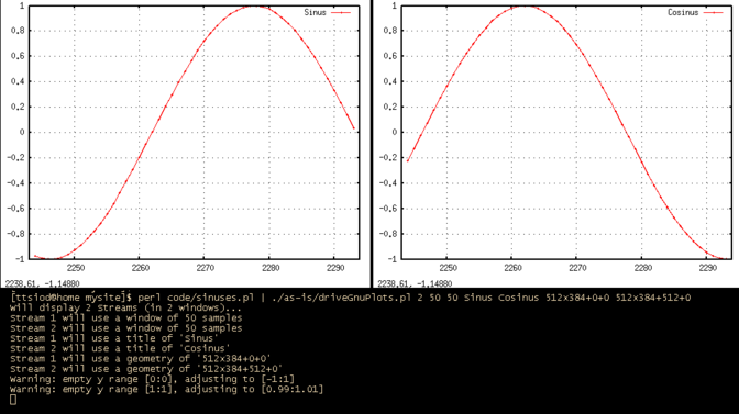
Preparing for a demo

You don't want to move the GnuPlot windows after they are shown, do you? So you can just specify their placement, in "WIDTHxHEIGHT+XOFF+YOFF" format (in pixels):

bash$ ./sinus.pl | ./driveGnuPlots.pl 2 50 50 Sinus Cosinus 512x384+0+0 512x384+512+0

The provisioning of titles and GnuPlot window placement information, makes the script very well-suited for live demonstrations.

P.S. UNIX power in all its glory: it took me 30min to code this, and another 30 to debug it. Using pipes to spawned copies of gnuplots, we are able to do something that would require one or maybe two orders of magnitude more effort in any conventional programming language (yes, even accounting for custom graph libraries - you do have to learn their API and do your windows/interface handling...)

Update, November 30, 2009: Andreas Bernauer has improved the script further, allowing multiple streams to be plotted in the same window. His work is here.

Update, December 20, 2009: Dima Kogan has done his own version, which detects the number of streams dynamically. He placed his code on GitHub.

Nomen est omen... main(O){10<putchar(6^--O?84-(31&0x20558400>>5*O):10)&&main(2+O);}

My CV About me Back to homepage

Last update on: Tue Nov 8 15:50:19 2011 (Valid HTML, Valid CSS)